This is a re-upload from my old site. But for anyone who has not seen it, or if you’re here to refresh that knowledge, here you go!
The thing that got me interested in Machine Learning was a course in college called Computational Intelligence. During the course we had a project on Genetic Algorithms that I found fascinating. Recently I found a reason to create one and I wanted to share it with you! These types of Algorithms can be quite confusing to implement, so I plan to walk through exactly how I created one. I will be referencing this book for anyone interested. Don’t feel like buying it but still want to use it? Check out research gate. Quick life pro tip: these types of academic books can often be acquired for free by requesting the publication from the author. Research gate allows you to do that! For each portion of the Genetic Algorithm I will describe the details followed by code implementing those details. Let’s get started!
This is going to be broken into the following sections, so feel free to skip to something if you don’t feel like reading the entire thing:
- What is a Genetic Algorithm?
- How Will this be Organized?
- What Can the Genetic Algorithm Optimize?
- Implementation
- What Can Genetic Algorithms Do?
- Conclusion
What is a Genetic Algorithm?
Before we dive into the programming portion, it is helpful to know what a Genetic Algorithm is. Genetic Algorithms model genetic evolution and were first developed to simulate genetic systems. Characteristics of individuals are expressed using genes and evolve over a number of generations. Individuals evolve through selection, crossover and mutation. These individuals live within a population and compete against one another so that the fittest ones survive.
How Will this be Organized?
Since I’m a big fan of Python, it will be written entirely in Python. If you’re following along or want to use this, you just need Python 3.6+ (I use 3.7) and numpy. If you need to install numpy, check out this link. This will be created as a Python module and split into files corresponding to the files’ individual functions.
What Can the Genetic Algorithm Optimize?
It can actually optimize a lot! For testing purposes and making the following sections easier to understand, I will use the three-hump camel function from this list of test functions. The three-hump camel function is modeled by the equation:
with a global minimum at $ f(0,0) = 0 $.
Implementation
Individual
First we need a way to represent the individual. There are two main ways to represent an individual: binary or floating-point. With binary representation you lay the chromosome out in a binary string and perform operations on slices of this string. Floating-point representation is different, it is just represented by the floating-point number. You could convert the floating-point number to binary but researchers have shown that using floating-point representation on floating-point problems yields better results. Because a chromosome is made up of several genes, we need a way to encode and decode the chromosome. In our case, the genes will be x and y, the two parameters to our three-hump camel function. I’m going to start by giving an abstract representation of an individual and later fully define these functions. Let’s code this!
# genetic_algorithm/Individual.py
from abc import abstractmethod
from typing import Optional, Union
import numpy as np

class Individual(object):
    def __init__(self):
        pass

    @abstractmethod
    def calculate_fitness(self):
        raise Exception('calculate_fitness function must be defined')

    @property
    @abstractmethod
    def fitness(self):
        raise Exception('fitness property must be defined')

    @fitness.setter
    @abstractmethod
    def fitness(self, val):
        raise Exception('fitness property cannot be set. Use calculate_fitness instead')

    @abstractmethod
    def encode_chromosome(self):
        raise Exception('encode_chromosome function must be defined')

    @abstractmethod
    def decode_chromosome(self):
        raise Exception('decode_chromosome function must be defined')

    @property
    @abstractmethod
    def chromosome(self):
        raise Exception('chromosome property must be defined')

    @chromosome.setter
    def chromosome(self, val):
        raise Exception('chromosome property cannot be set.')
This is a good abstract outline for an individual. It will require further implementation, but for now it will suffice. It lays a foundation for what all individuals in any Genetic Algorithm need: a way to calculate fitness, encoding and decoding of the chromosome.
Population
Now that we have an individual defined, we need a way to define the overall population. The population is really just a collection of individuals that will compete against each other. For this we really just need to keep track of the best individual, average fitness, number of genes and any other statistical information we want. Let’s code this!
# genetic_algorithm/Population.py
import numpy as np
from typing import List
from .individual import Individual


class Population(object):
    def __init__(self, individuals: List[Individual]):
        self.individuals = individuals

    @property
    def num_individuals(self) -> int:
        return len(self.individuals)

    @num_individuals.setter
    def num_individuals(self, val) -> None:
        raise Exception('Cannot set the number of individuals. You must change Population.individuals instead')

    @property
    def num_genes(self) -> int:
        return self.individuals[0].chromosome.shape[1]

    @num_genes.setter
    def num_genes(self, val) -> None:
        raise Exception('Cannot set the number of genes. You must change Population.individuals instead')

    @property
    def average_fitness(self) -> float:
        return np.mean(np.array([individual.fitness for individual in self.individuals]))

    @average_fitness.setter
    def average_fitness(self, val) -> None:
        raise Exception('Cannot set average fitness. This is a read-only property.')

    @property
    def fittest_individual(self) -> Individual:
        return max(self.individuals, key = lambda individual: individual.fitness)

    @fittest_individual.setter
    def fittest_individual(self, val) -> None:
        raise Exception('Cannot set fittest individual. This is a read-only property')

    def calculate_fitness(self) -> None:
        for individual in self.individuals:
            individual.calculate_fitness()

    def get_fitness_std(self) -> float:
        return np.std(np.array([individual.fitness for individual in self.individuals]))
Selection
If you have the Computational Intelligence book that I linked at the beginning, this comes from section 11.2.2 Selection Operators. Selection operators exist to determine which individuals survive to the next generation. In a lot evolutionary programming, selection is done from both parents and offspring. This allows for offspring to be created without the fear you will lose good genetic information from the parent. Some Algorithms will keep the top n parents and then perform crossover from top and/or random individuals until you each a number of offspring. There are a number of ways to tweak Genetic Algorithms, so if you are ever curious what would happen by changing x, the best advice I can give is to just try it. Machine Learning after all is a science and a great way to gain intuition in science is by trying!
The three selection operators I will focus on are: elitism, tournament and roulette wheel. Elitism is picking the top n individuals from a given population. This is why the fitness function matters. Individuals share the same fitness function and can then be judged based off of their fitness. Tournament selection is like elitism, but within smaller tournament sizes. Each time you will select a tournament size, k, and from within that tournament, select the top individual. You repeat this until you get n individuals. This allows for more diversity if the tournament size is small. Finally we have the roulette wheel. We can create a giant wheel where each slice of the wheel is an individuals fitness. If we spin the wheel, we have a higher probability of landing on one of the more fit individuals, but we still have a probability to select a low performing individual. This concept can really help with exploration, which I will explain later. Let’s code these three selection operators!
# genetic_algorithm/Selection.py
import numpy as np
from typing import List
from .population import Population
from .individual import Individual


def ellitism_selection(population: Population, num_individuals: int) -> List[Individual]:
    individuals = sorted(population.individuals, key = lambda individual: individual.fitness, reverse=True)
    return individuals[:num_individuals]

def roulette_wheel_selection(population: Population, num_individuals: int) -> List[Individual]:
    selection = []
    wheel = np.sum(individual.fitness for individual in population.individuals)
    for _ in range(num_individuals):
        pick = np.random.uniform(0, wheel)
        current = 0
        for individual in population.individuals:
            current += individual.fitness
            if current > pick:
                selection.append(individual)
                break

    return selection

def tournament_selection(population: Population, num_individuals, tournament_size: int) -> List[Individual]:
    selection = []
    for _ in range(num_individuals):
        tournament = np.random.choice(population.individuals, tournament_size)
        best_from_tournament = max(tournament, key = lambda individual: individual.fitness)
        selection.append(best_from_tournament)

    return selection
Crossover
We now have a way to model an individual, express a population and select individuals based off their fitness. Next we need a way to have two individuals reproduce. A common crossover method for binary represented individuals is single point crossover. With single point crossover you select a random point in the gene and swap data. Because we are using floating-point representation, single point binary crossover won’t work. We can, however, use simulated binary crossover (SBX). SBX generates offspring symmetrically around the parents. This helps prevent any bias towards either parent. From the Computational Intelligence book it is described as: “Two parents, $ x_{1}(t) $ and $ x_{2}(t) $ are used to produce two offspring, where $ j=1, …, n_{x} $
where
where $ r_j \sim U(0, 1), \text{and } \eta > 0 $ … For large values of $ \eta $ there is a higher probability that offspring will be created near the parents. For small $ \eta $, offspring will be more distant from the parents.”
So what does this all mean? Well, this is just fancy math speak for: create a random uniform variable between [0, 1), and if that variable is $ \geq 0.5 $, assign $ \gamma $ one value, otherwise assign it the other value based off equation 9.11. Once you have a value for $ \gamma $, create two offspring genes, \(\tilde{x}_{1}(t) \text{ and } \tilde{x}_{2}(t)\).
Repeat this for every gene in the chromosome to create two child chromosomes. Because of numpy syntax, we don’t actually need a single for loop. I know this might still seem confusing so let’s code this and compare again!
# genetic_algorithm/Crossover.py
import numpy as np
from typing import Tuple
from .individual import Individual


def simulated_binary_crossover(parent1: Individual, parent2: Individual, eta: float) -> Tuple[np.ndarray, np.ndarray]:
    # Calculate Gamma (Eq. 9.11)
    rand = np.random.random(parent1.chromosome.shape)
    gamma = np.empty(parent1.chromosome.shape)
    gamma[rand <= 0.5] = (2 * rand[rand <= 0.5]) ** (1.0 / (eta + 1))  # First case of equation 9.11
    gamma[rand > 0.5] = (1.0 / (2.0 * (1.0 - rand[rand > 0.5]))) ** (1.0 / (eta + 1))  # Second case

    # Calculate Child 1 chromosome (Eq. 9.9)
    chromosome1 = 0.5 * ((1 + gamma)*parent1.chromosome + (1 - gamma)*parent2.chromosome)
    # Calculate Child 2 chromosome (Eq. 9.10)
    chromosome2 = 0.5 * ((1 - gamma)*parent1.chromosome + (1 + gamma)*parent2.chromosome)

    return chromosome1, chromosome2
As you can see, the first section is just setting gamma, \gamma , based off equation 9.11. It may not be apparent, but we can use numpy syntax to actually create a multi-dimensional array with the same shape as the chromosome. Since the chromosome is a collection of genes, this is really creating a gamma value for each gene. This allows for genes from one chromosome to crossover with genes from another. The second part is applying the gamma (multi-dimensional array) to the parents and creating two chromosome offspring.
Mutation
Mutation is the act of introducing variation in an Evolutionary Program. Because of this, mutation plays a very important role in the exploration-exploitation trade off. From the Computational Intelligence book, mutation is defined as:
This just says you create some offspring \(x^{'}_{i}\) from parent $ x_{i}(t) $ by adding variation $ \Delta x_{i}(t) $. The only thing that changes between different mutation Algorithms is how you calculate $ \Delta x_{i}(t) $. I am going to focus on a non-adaptive form, which means the deviations remain static. That is, over time there will not be a scaling attribute applied to $ \Delta x_{i}(t) $. It can be helpful to have a scaling function that adapts over time but it can also add more complexity. In this case I want to focus on what mutation can do and I find using non-adaptive scaling is best for this. If you’re curious about other types of scaling, I would recommend reading section 11.2 from the Computational Intelligence book. Normally I wouldn’t just say, “go read this”, but I think discussing the scaling parameter is out of the scope for this blog post.
Although there are many variations to mutation, the three I will focus on are Gaussian, uniform and uniform with respect to the best individual. Gaussian mutation will center the mean around some variable, $ \mu $, with standard deviation, $ \sigma $. This means you can say:
Because the Gaussian mutation is adding noise, we can set $ \mu_{ij}(t) = 0 $ the majority of the time. This will allow for both positive and negative values of noise being added to an individual. With uniform mutation you have:
We don’t actually need to assign this to $ \Delta x_{ij}(t) $, but can instead assign it directly to the offspring, $ x^{‘}_{ij}(t) $.
Uniform mutation with respect to the fittest individual is very similar:
where $ \hat{y}(t) $ is the best individual from the current population. Let’s code these!
# genetic_algorithm/Mutation.py
import numpy as np
from typing import List, Union
from .individual import Individual


def gaussian_mutation(individual: Individual, prob_mutation: float,
                      mu: List[float] = None, sigma: List[float] = None) -> None:
    """
    Perform a gaussian mutation for each gene in an individual with probability, prob_mutation.

    If mu and sigma are defined then the gaussian distribution will be drawn from that,
    otherwise it will be drawn from N(0, 1) for the shape of the individual.
    """
    chromosome = individual.chromosome
    # Determine which genes will be mutated
    mutation_array = np.random.random(chromosome.shape) < prob_mutation
    # If mu and sigma are defined, create gaussian distribution around each one
    if mu and sigma:
        gaussian_mutation = np.random.normal(mu, sigma)
    # Otherwise center around N(0,1)
    else:
        gaussian_mutation = np.random.normal(size=chromosome.shape)
    # Update
    chromosome[mutation_array] += gaussian_mutation[mutation_array]

def random_uniform_mutation(individual: Individual, prob_mutation: float,
                            low: List[float], high: List[float]) -> None:
    """
    Randomly mutate each gene in an individual with probability, prob_mutation.
    If a gene is selected for mutation it will be assigned a value with uniform probability
    between [low, high).
    """
    chromosome = individual.chromosome
    mutation_array = np.random.random(chromosome.shape) < prob_mutation
    uniform_mutation = np.random.uniform(low, high, size=chromosome.shape)
    chromosome[mutation_array] = uniform_mutation[mutation_array]

def uniform_mutation_with_respect_to_best_individual(individual: Individual,
                                                     best_individual: Individual,
                                                     prob_mutation: float) -> None:
    """
    Ranomly mutate each gene in an individual with probability, prob_mutation.
    If a gene is selected for mutation it will nudged towards the gene from the best individual.

    """
    chromosome = individual.chromosome
    best_chromosome = best_individual.chromosome
    mutation_array = np.random.random(chromosome.shape) < prob_mutation
    uniform_mutation = np.random.uniform(size=chromosome.shape)
    delta = (best_chromosome[mutation_array] - chromosome[mutation_array])
    chromosome[mutation_array] += uniform_mutation[mutation_array] * delta
Exploration vs. Exploitation
Now it’s time to discuss exploration vs. exploitation. Exploration is generally done earlier on in Algorithms. Exploration is the act of searching around to find other possible routes. If you were to only search one area, you may end up in a local maxima, whereas if you explore you can check out multiple areas at the same time. As time progresses you will often find one of your explorations leads to better fitness, at which time you will want to exploit that area. Exploitation means fine tuning until you find the optimal value. Because mutation helps with exploration, it may be beneficial to begin with a 5% mutation rate and lower it as the generations increase. This will allow for more mutation earlier on while focusing on crossover in later generations, which may lead to better results!
Designing the Individual
Each problem is going to be slightly different, meaning the Genetic Algorithm will need to be changed for that problem. Because of how I laid the foundation, the only thing that needs to be added is an individual for the problem. So what is the problem? The three-hump camel function! We can use the fact that the global minimum is at $ f(0, 0) = 0 $ to evaluate how well our Genetic Algorithm performs! Let’s take a quick look at this function and then I’ll explain why I create the individual in a certain way:
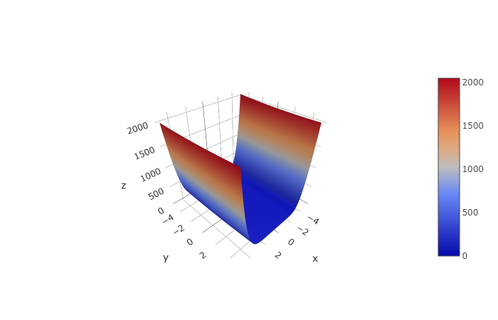
$ \text{from }-5 \leq x, y \leq 5 $
You can see how drastic the values change on the outer edges and how fine tuning will be required to find the minimum. Let’s see what an individual for this problem would look like!
# func_individual.py
import numpy as np
from typing import Optional
from genetic_algorithm.individual import Individual


three_hump_camel_func = lambda x,y: (2*x**2 - 1.05*x**4 + ((x**6)/6) + x*y + y**2)

class FunctionIndividual(Individual):
    def __init__(self, chromosome: Optional[np.ndarray] = None):
        super().__init__()
        # Is chromosome defined?
        if not chromosome is None:
            self._chromosome = chromosome
            self.decode_chromosome()
        else:
            self.x = np.random.uniform(-5, 5)
            self.y = np.random.uniform(-5, 5)
            self.encode_chromosome()

        # Default value. It is important to call calculate_fitness in order
        # to get the real fitness value
        self._fitness = -1e9

    def calculate_fitness(self):
        self._fitness = 1. / three_hump_camel_func(self.x, self.y)

    @property
    def fitness(self):
        return self._fitness

    def encode_chromosome(self):
        self._chromosome = np.array([self.x, self.y], dtype='float')

    def decode_chromosome(self):
        self.x = self._chromosome[0]
        self.y = self._chromosome[1]

    @property
    def chromosome(self):
        return self._chromosome
One thing you might notice is the calculate_fitness function sets the fitness to 1. / three_hump_camel_func(self.x, self.y) and this might seem a bit strange at first. Remember that we want the most fit individual to survive. Because the global minimum is at $ f(0, 0) = 0 $ we don’t want the fitness to be defined by just the output of the function as this would reward individuals further from the global minimum. If the goal is to find the global minimum, we can instead set it to 1. / fitness. As individuals get closer to $ f(0, 0) $, their fitness will approach infinity. Another thing you may notice is how I defined the chromosome for the individual. Because this problem lives in three-dimensional space and evaluated through $ f(x, y) $, I have chosen to give the individual two genes, $ x $ and $ y $, which make up the chromosome. The encode_chromosome will create a chromosome from the individuals’ genes and the decode_chromosome will split the chromosome back into the individuals’ genes.
Putting it Together
If you are curious, take a look at Algorithm 12.1 Evolution Strategy Algorithm from the Computational Intelligence book. Below is my take on this Algorithm, where $ \mu $ indicates the number of parents and $ \lambda $ the number of offspring:
I’m going to tweak it a bit for my implementation. I’m going to bring the top two individuals from the previous generation (elitism), always have 60 individuals in the population and evaluate fitness at the beginning of a generation. In this problem it does not matter when you evaluate the fitness. In other problems, however, you may not be able to immediately evaluate the fitness. Take for example a paper airplane: you can’t create one and know how it will perform; you need to throw it before you can evaluate it. Let’s code it!
# test_ga.py
import numpy as np
import matplotlib.pyplot as plt
from math import sqrt
import random
from func_individual import FunctionIndividual, three_hump_camel_func
from genetic_algorithm.individual import Individual
from genetic_algorithm.population import Population
from genetic_algorithm.selection import elitism_selection, roulette_wheel_selection, tournament_selection
from genetic_algorithm.crossover import simulated_binary_crossover as SBX
from genetic_algorithm.mutation import gaussian_mutation

np.random.seed(0)
random.seed(0)
NUM_INDIVIDUALS = 60
NUM_GENERATIONS = 300

def genetic_algo():
    fitness = []  # For tracking average fitness over generation

    # Create and initialize the population
    individuals = [FunctionIndividual() for _ in range(NUM_INDIVIDUALS)]
    pop = Population(individuals)

    # Calculate initial fitness
    for individual in pop.individuals:
        individual.encode_chromosome()
        individual.calculate_fitness()

    for generation in range(NUM_GENERATIONS):
        next_pop = []  # For setting next population

        # Decode the chromosome and calc fitness
        for individual in pop.individuals:
            individual.decode_chromosome()
            individual.calculate_fitness()

        # Get best individuals from current pop
        best_from_pop = elitism_selection(pop, 2)
        next_pop.extend(best_from_pop)

        while len(next_pop) < NUM_INDIVIDUALS:
            # p1, p2 = roulette_wheel_selection(pop, 2)
            p1, p2 = tournament_selection(pop, 2, 4)
            mutation_rate = 0.05 / sqrt(generation + 1)
            # mutation_rate = 0.05

            # Create offpsring through crossover
            c1_chromosome, c2_chromosome = SBX(p1, p2, 1)
            c1 = FunctionIndividual(c1_chromosome)
            c2 = FunctionIndividual(c2_chromosome)

            # Mutate offspring
            gaussian_mutation(c1, mutation_rate)
            gaussian_mutation(c2, mutation_rate)

            # Add to next population
            next_pop.extend([c1, c2])

        # Track average fitness
        fitness.append(pop.average_fitness)

        # Set the next generation
        pop.individuals = next_pop

    plt.yscale('symlog')
    plt.xlabel('Generation')
    plt.ylabel('Fitness')
    plt.plot(range(len(fitness)), fitness)
    plt.tight_layout()
    plt.show()

genetic_algo()
Here is the average fitness of the population over the generations:
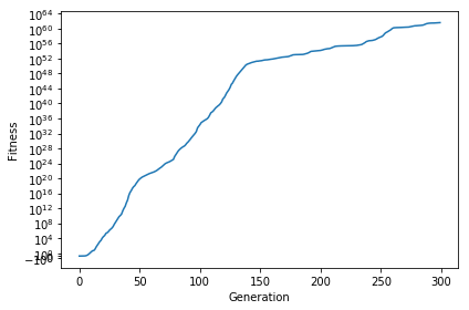
And that’s it! That wasn’t too bad, was it? The majority of the code is really defining selection, mutation and crossover methods. Describing an individual doesn’t take too long once you have an abstract outline and most Genetic Algorithms follow the same pattern. What I mean is you could easily define a new individual for a different problem and plug it into the same code above and it would be able to help optimize! You could even just switch which function you want to find the minimum/maximum of and only need to change calculate_fitness, encode_chromosome and decode_chromosome. You may notice I commented out some code in the above section. I talked previously about exploration vs. exploitation and how you may want to use a decaying mutation rate so you can focus on exploration earlier on, while prioritizing exploitation as generations increase. You should also consider the fact that the y-axis is logarithmic. This shows how the Genetic Algorithm can perform small changes to continue improving the average fitness of the population!
Below is a gif showing the difference between using tournament selection with 5% mutation, tournament selection with decaying mutation, roulette wheel selection with 5% mutation and roulette wheel with decaying mutation. All of these Algorithms are given the same starting population, the only thing that changes is the selection operator and mutation rate. Let’s see how they compare over 300 generations!
One thing to notice is how Roulette + Decaying actually converges to a local minima for the first 30 generations, but because of exploration, is able to find the global minimum around generation 40. You can also see that the populations with decaying mutation rates have a lot less “noise” in the later generations. This is because exploration is what causes the noise in the first place. Since the decaying mutation puts less emphasis on exploration as the generations increase, you will get the population converging to a specific area. You can also see how the populations with the 5% mutation have a lot more exploration even at the later generations, even though the majority of the population continues to converge to the global minimum of $ f(0, 0) = 0 $. It is also important to realize that these populations have 60 individuals each! That means for the majority of the population, most individuals are at the global minimum.
What Can Genetic Algorithms Do?
Above I really only showcased a Genetic Algorithm being able to find a global minimum of a three-dimensional function, but they can do so much more! Genetic Algorithms work well in environments where you may not be able to take a derivative or may not have data to train on. I have talked before about how Neural Networks use backpropagation to figure out what the weights should be. This is done by giving the Network a set of training data to train on, comparing against the current output and updating weights accordingly. If, however, you don’t have training data, you could use a Genetic Algorithm to help figure out what those weights should be! I used this technique to create an AI that learns to play Super Mario Bros.
Conclusion
In this post we took a look at what a Genetic Algorithm can do and referenced a Computational Intelligence book to bring these ideas to Python. We were able to take a three-dimensional function with local minima and compare how different populations behave while trying to find the global minimum. I showed that once you have an outline for the Genetic Algorithm, the only thing you really need to do is define the individual for a given problem. Although finding a global minimum might not seem the most exciting, I believe it lays a good foundation for solving future, more complex problems! Genetic Algorithms are also what first got me so excited about Machine Learning and I wanted to share it with you. As always, if you have feedback, please let me know. Whether you loved the content or hated it, all feedback is welcome. Feel free to share this with anyone who might also find this interesting!