The video is ready! If you want to see a YouTube video of the different accomplishments of these AI, take a look here.
Update: These AI were able to complete worlds 1-1, 2-1, 3-1, 4-1, 5-1, 6-1, and 7-1. They were also able to learn to do a walljump, flagpole glitch, and fast acceleration. World 8-1 has not been completed…. yet.
Before we dive in, let me just start by saying there are many different ways to have an AI learn an environment. In the last decade huge advancements have been made in this field that address many of the issues faced when creating an AI. In future posts I will get into some of these advancements, but first it’s important to understand why they were needed. In this post I’m going to show how to use a genetic algorithm and a neural network to solve Super Mario Bros, and why it’s not the best choice to do so. This is going to be a long one. So sit back, relax with your favorite beverage, and enjoy. Hopefully this can whet your appetite for what’s to come.
This is going to be broken into the following sections, so feel free to skip to something if you don’t feel like reading the entire thing:
- Why Use a Genetic Algorithm?
- Why Use a Neural Network?
- What is a State?
- Reading RAM Values
- Discriminate Between States
- Generalize Within States
- Defining a Fitness Function
- Bringing Everything Together
- Seeing it in Action
- Results
- Limitations of Genetic Algorithms
Why Use a Genetic Algorithm?
Genetic algorithms are good at searching high dimensional problem spaces. A lot of times this is where people get confused and that’s fair. As humans we don’t think in high dimensional spaces. So let’s start small.
Let’s say that we want to find the maximum of a function, \(y = x\). Another way to write this is to find the maximum of \(f(x)\) where \(f\) is just a function that maps \(x\) onto \(y\).
Here, \(f\) would just assign \(y = x\). If we bound parameters between \([-5, 5]\), then the maximum would be at \(x = 5\). This would be a one dimensional problem since we are finding the best value over one parameter, \(x\). Generally we see this as a two dimensional graph since we usually plot \(y\) along with \(x\) but in this case we will consider \(f(x)\) to be one dimensional. If we want to maximize a two dimensional problem, then we are maximizing \(f(x, y)\). Because of the way I created define the environment, Mario became a 789 dimensional problem. This means that I’m maximimizing over \(f(x_{1}, x_{2}, ..., x_{789})\), where each \(x\) is a parameter. I’ll get into what exactly the parameters are in a little bit.
Why Use a Neural Network?
Neural networks are really good function approximators. I just talked about maximizing a function, but it’s important to remember that a function \(f(x) = 2x\) is mapping the output to be equal to \(2x\) the input. So what if you don’t have this mapping? What if you don’t have a function? You can use a neural network to approximate values. Consider this:
We could take many samples and have a neural network learn a function to map the inputs onto outputs. Because we would like a way to map Mario’s state onto actions, we would like to find a function, \(action = f(state)\), where \(state\) is the input, and an \(action\) is the output. Obviously if we just had a magic function, \(f(state)\), then we could just plug in Mario’s \(state\) and know the exact \(action\) to take, and this is ultimately what we want.
What is a State?
We know that we want to find a magic function, \(f(state)\) that tells us what \(action\) to take, but how do we describe a \(state\)? There is actually a lot of thought that goes into this. No matter what the problem, describing the set of states can make you solve a problem quickly or never solve it at all. We want a state to be able to describe the environment Mario is currently dealing with.
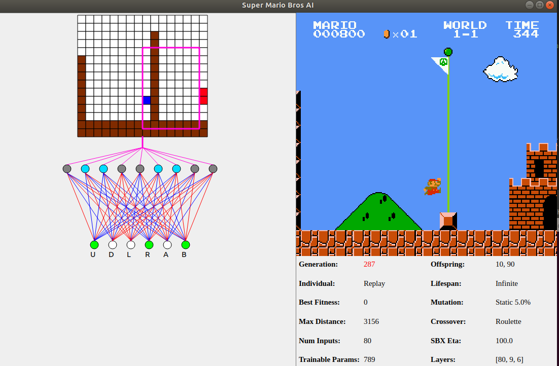
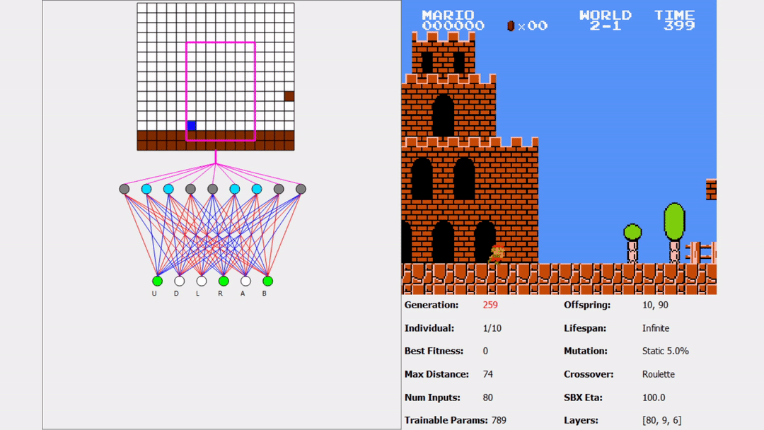
For this I will be splitting the screen into a 13x16 matrix consisting of blocks. Because this game is on the Nintendo Entertainment System (NES), there are some very limited graphics that help make this choice obvious. Everything you see in Super Mario Bros is really just made up of a bunch of blocks. Mario? Block. Goomba? Block. Flag pole? Many blocks. Even the bushes are blocks of background graphics. All the blocks on the screen make up a 13x16 grid for a total of 208 blocks.
The next question that might come to mind is which blocks actually matter? Should we use all of the blocks or just a small section? We could let the AI choose which blocks are most important but we don’t necessarily need to. When I’m playing Mario I rarely look behind me. In fact, my strategy is really just “run right and jump”. If you take a look at the original photo you will notice a pink box. That is the region of blocks I chose for Mario to use to help decide the set of states. I’ll discuss why and how this came to be toward the end. For now it’s only important to know that the blocks within that pink rectangle are what matter.
Reading RAM Values
Random Access Memory (RAM) is a good place for storing data. Computers use RAM all the time to store data that is frequently accessed or currently being used. Video games also use RAM, and in this case we are going to use that knowledge to read values we care about and help build upon describing the \(state\). We know a state describes the current environment and we know that the screen is made up of a 13x16 grid of blocks. What we need now is a way to get this grid. That is where RAM comes in. I used the information found here to decide what information I actually cared about. Here is an example of how to access RAM using OpenAI Retro:
import retro
env = retro.make(game='SuperMarioBros-Nes', state='Level1-1')
env.reset()
ram = env.get_ram()
From here, using the RAM map, we can access any information that we want. Figuring out how far Mario has made it through the level becomes as easy as:
distance_traveled = ram[0x006D]
I do this same technique to grab Mario’s distance through the level, current position on screen, enemy positions on screen, etc. If you want to see how this works in code you can take a look at at a helper module I wrote here. For anyone that does, you may notice that the resolution of the NES is actually 240x256 (this is normally written as 256x240, but I’m writing it the other way to keep the same syntax as the grid). Since the sprite blocks are all 16x16 you might realize that the block grid should be 15x16, not 13x16, and you’d be right. There technically are 2 rows that I ignore when looking at the blocks and that is because the NES Picture Processing Unit (PPU) actually doesn’t scroll through that section, so the blocks are always empty there. This can be seen below (gif taken from here):
Notice how the score, number of coins, world, and time are not shown. That’s loaded differently and because of that, I can treat the top two rows as being empty. Now we need to actually decide what blocks are important.
Blocks can take values between \([0x00, 0xFF]\). It may be temping to want to use all values so that you can get a full range of possible inputs. One reason I don’t just treat each pixel as an input for our \(state\) is I don’t want to have 61,440 inputs (240x256 resolution). In this case, if I consider 70 blocks, then each of those blocks can take on values 0 through 255 (0xFF). Because of how the neural network operates, larger input values will represent a strong intensity. There really shouldn’t be a stronger intensity for a block with value 100 compared to a block with value 6, especially if block 6 is really bad for Mario and block 100 is a star. Because of this, it would be better to encode the data somehow. One popular method of doing so is called one-hot encoding, where you create a vector of length \(k\) for \(k\) different objects and put a \(1\) in the location of the object and \(0\) elsewhere. Below is an example:
colors = ['red', 'yellow', 'green']
one_hot_red    = [1, 0, 0]
one_hot_yellow = [0, 1, 0]
one_hot_green  = [0, 0, 1]
This makes it so we can treat all blocks with equal intensity, however, now we would have 17,920 (70 blocks * 256 block values) inputs. Although this is better, it’s still not ideal.
Let’s see what these RAM values look like to get a better understanding:
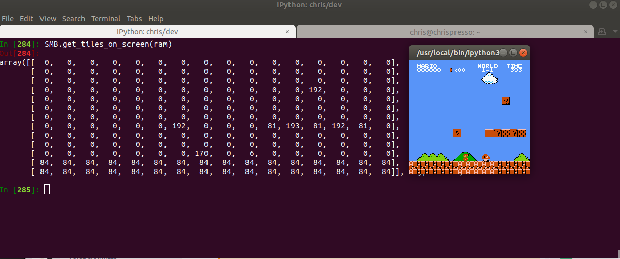
In this case I added the value 170 (0xAA) to represent where Mario is on the screen. Instead of representing a full range of values of blocks, we can instead focus on what we actually care about. Is the block safe, an enemy or empty? Empty blocks just have a value of \(0\), so there’s nothing that needs to be done there. For safe vs. enemy blocks it gets a little more complicated. There are enemy blocks and static blocks, so it’s possible that values overlap. Because of this, it is necessary to look at the enemy locations in RAM and see if any of them are on the screen. Since Super Mario Bros can only draw 5 enemies at a time, code to find enemies on screen looks something like this:
import numpy as np
from collections import namedtuple

Point = namedtuple('Point', ['x', 'y'])
# Set bins. Blocks are 16x16 so we create bins offset by 16
ybins = list(range(16, 240, 16))
xbins = list(range(16, 256, 16))

def get_enemy_locations(RAM):
    enemy_locations = []

    for enemy_num in range(5):
        enemy = RAM[0xF + enemy_num]
        # RAM locations 0x0F through 0x13 are 0 if no enemy
        # drawn or 1 if drawn to screen
        if enemy:
            # Grab the enemy location
            x_pos_level  = RAM[0x6E + enemy_num]
            x_pos_screen = RAM[0x87 + enemy_num]
            # The width in pixels is 256. 0x100 == 256.
            # Multiplying by x_pos_level gets you the
            # screen that is actually displayed, and then
            # add the offset from x_pos_screen
            enemy_loc_x = (x_pos_level * 0x100) + x_pos_screen
            enemy_loc_y = RAM[0xCF + enemy_num]
            # Get row/col
            row = np.digitize(enemy_loc_y, ybins)
            col = np.digitize(enemy_loc_x, xbins)
            # Add location.
            # col moves in x-direction
            # row moves in y-direction
            location = Point(col, row)
            enemy_locations.append(location)

    return enemy_locations
This will get us all enemies that are present on the screen and their block locations. We can set the block values of these locations to \(-1\). All that we need to do now is get the locations of remaining blocks and set them to \(1\). I won’t be posting code for this, but you can check out get_tiles under utils if you’re curious how this is done.
Now we have a way to represent a block as either \(\{-1, 0, 1\}\) for enemy, empty, or safe, respectively. We could use one-hot encoding on these three type of blocks, but instead we can just use the value. The reason this is possible is because the values will no longer represent a strong/weak intensity. This means instead of using 17,920 inputs for 70 blocks, we only need 70 blocks, which is much better.
Discriminate Between States
Now we have a way to desribe values for blocks, so how do we describe the state? Well, the state is just made up of the collection of blocks. In this case we can have \(n\) blocks and 3 values for each block for a total of \(3^{n}\) possible states. Of course, not all states are actually possible. I already said Super Mario Bros can only draw 5 enemies at once, so there is no way for there to be a value of \(-1\) at all blocks. This is another reason that using a neural network is important. Rather than having a giant lookup table, \(f\), that maps from \(state\) to \(action\), we can use the neural network to approximate what \(action\) to take.
Once a value in one of the blocks changes, the state changes. This is the way we discriminate between states. If Mario is standing still and the environment isn’t changing, then the \(state\) is the same the entire time.
Generalize Within States
If we were to use pixel values then there would be \(256^{3}\) pixel values (256 red, 256 green, and 256 blue). If you generalize at a \(1x1\) pixel level, then anytime Mario moves a single pixel, Mario would enter a new state. If you used the entire screen you would have \(num\_values^{screen\_size}\), which becomes \((256^{3})^{256*240} \approx 6.17 * 10^{443,886}\). Luckily we don’t do that, and instead we are using blocks. Because of this, even if Mario moves 8 pixels in a direction, the block will still generalize within the same \(state\). This is helpful since it doesn’t really matter if something moves slightly. I know this might seem confusing, but just remember that generalization within a \(state\) is important.
Defining a Fitness Function
Genetic algorithms work by deciding which individuals are the most fit and basically giving them a probability that they will reproduce. So how do we decide what this fitness function should be? Let’s say we define a fitness function that looks like this:
def fitness(distance):
    return distance
In this case each individual has a fitness related to how far it moved. But what if \(individual_{1}\) took 60 seconds to get \(distance=100\) and \(individual_{2}\) took 5 hours to get \(distance=100\), should they have the same fitness? Probably not. One way to get around this is to track the amount of time that an individual was alive for, and subtract it from the overall fitness. Now we could have something that looks like:
def fitness(frames, distance):
    return distance - frames
One problem with this is \(distance\) is treated linearly, but we really want to emphasize reward for the individual moving further through the level. We can add some exponential to address this, like so:
def fitness(frames, distance):
    return distance**1.9 - frames**1.5
Because individuals aren’t moving a lot in the beginning, we really want to reward the early explorers that do begin moving, increasing their probability to reproduce. This could look something like this:
def fitness(frames, distance)
    return distance**1.9 - frames**1.5 +\
           min(max(distance - 50, 0), 1) * 2000
Now early explorers that make it past \(distance=50\) receive an additional reward of \(2000\). But should we also reward individuals that actually beat the level? If the finish is at \(distance=4000\) and there is an individual that stop at \(distance=3980\), we don’t want that individual to have a nearly identical fitness as individuals that actually complete the level. Below is code to take that into consideration:
def fitness(frames, distance, did_win)
    return distance**1.9 - frames**1.5 +\
           min(max(distance - 50, 0), 1) * 2000 +\
           did_Win * 1e6
This type of thinking can continue forever. It can be best to test several fitness functions and see how the different populations evolve due to these differences. Here is an actual example of a fitness function I used to test a population:
def fitness(frames, distance, game_score, did_win):
    return max(distance ** 1.9 - \
           frames ** 1.5 +   \
           min(max(distance-50, 0), 1) * 2000 + \
           game_score**2 + \
           did_win * 1e6, 0.00001)
Take a look at that and think about what could happen and what the individuals will learn to prioritize. If you need a hint, take a look at this one and try to find the difference:
def fitness(frames, distance, game_score, did_win):
    return max(distance ** 1.9 - \
           frames ** 1.5 +   \
           min(max(distance-50, 0), 1) * 2000 + \
           game_score * 20 + \
           did_win * 1e6, 0.00001)
Bringing Everything Together
I know the stuff I described above will most likely seem confusing. That’s okay! It took me a long time to wrap my head around genetic algorithms. So I know throwing all of this at you at once might seem like a lot. Let’s break it down to describe the main concepts and how they are linked:
- Because we have a large state space I generalize the states into 16x16 pixel blocks.
- Determine which blocks should have values \(\{-1, 0, 1\}\)
- The goal is to have a function \(f(state)\) that outputs what \(action\) to take.
- We can’t use a lookup table because:
- This table would have \(3^{num\_blocks}\) entries.
- We don’t have a lookup table for this.
- Because we can’t use a lookup table, we use a neural network to approximate \(f(state)\) that we wish to learn.
- The genetic algorithm will be used to find parameter values for the neural network that maximizes fitness.
- Individuals are more likely to reproduce, and spread their parameter values, based on their fitness.
- Because reproduction is a probability, even less fit individuals have a chance to reproduce. This helps with genetic diversity.
- Crossover of these parameters are a gaussian distribution around parent parameters to help keep genetic diversity.
- As the genetic algorithm improves these parameters, the function approximation of \(f(state)\) improves.
Below is some pseudocode to accomplish this:
    \begin{algorithm}
    \caption{Genetic Algorithm with Neural Network}
    \begin{algorithmic}
    \STATE \textbf{Require:}
    \STATE Number of parents, $N_{p}$
    \STATE Number of children, $N_{c}$
    \STATE Neural Network size, $[L_{1}, L_{2}, ..., L_{N}]$
    \STATE Selection type, $S_{type}$
    \STATE Crossover type, $C_{type}$
    \STATE Mutation type, $M_{type}$
    \STATE
    \COMMENT{Initialize parent parameters randomly}
    \FOR {$i = 1$ \TO $N_{p}$}
        \FOR {$l = 2$ \TO $length(L)$}
            \STATE $\phi^{w_{l}}_{i} = U(-1, 1, size=(L[l], L[l-1]))$
            \STATE $\phi^{b_{l}}_{i} = U(-1, 1, size=(L[l], 1))$
        \ENDFOR
        \STATE Create Neural Network, $F_{i}$, from weights, $\phi^{w}_{i}$, and bias, $\phi^{b}_{i}$
    \ENDFOR
    \STATE Set number of individuals, $N_{ind} = N_{p}$
    \WHILE {$1$}
        \FOR {$ind = 1$ \TO $N_{ind}$}
            \STATE Get individual parameters, $\phi_{ind}$
            \WHILE {$alive(ind)$}
                \STATE Observe state, $S$
                \STATE Select action, $A = F_{ind}(S, \phi_{ind})$
            \ENDWHILE
            \STATE Calculate fitness, $fitness_{ind}$
        \ENDFOR
        \STATE Select any parents to carry over through $S_{type}$
        \STATE Set $next\_gen\_size$ according to $C_{type}, N_{p},$ and $N_{c}$
        \STATE Perform crossover according to $C_{type}$
        \STATE Perform mutation according to $M_{type}$
        \STATE Set $N_{ind} = next\_gen\_size$
    \ENDWHILE
    \end{algorithmic}
    \end{algorithm}
This syntax might seem a bit confusing, especially if you haven’t seen much pseudocode before. There is a reason I’m choosing to use certain syntax such as \(\phi\), which will become apparent in later blogs. Don’t get too hung up on the syntax. In fact it might help to ignore the syntax for parameters and just read what is happening on each line.
For this, \(\phi\) symbolizes the parameters of the neural network. Remember in the beginning where I said I’m maximizing over 789 parameters? These are those parameters. The genetic algorithm is what changes the parameters, and those parameters are what allow Mario to choose \(action = f(state)\). Those actions then get Mario a certain distance in the level, which in turn gives a fitness. That fitness allows the genetic algorithm to make changes to the parameters through selection, crossover, and mutation. This is really all the above pseudocode does. See? It’s not so bad!
One thing I should mention is I also used a one-hot encoding scheme for Mario’s row within the pink box. I tested both with and without the one-hot encoding for the row, but I found it helpful in certain situations. For instance, without it, Mario may see an enemy and jump. If Mario is already above the enemy, then there is no reason to jump. The one-hot encoding for the row helps Mario make these types of decisions. Another thing to realize is that everything within the pink box is an input to Mario’s neural network. I’m choosing not to display which input nodes are active because otherwise that would distract from what type of blocks are in each of those locations.
Seeing it in Action
Here is an in depth video showcasing all of what Mario was capable of learning.
Results
All AI discussed in this section were trained using the same fitness function:
def fitness(frames, distance, did_win):
    return max(distance ** 1.8 - \
           frames ** 1.5 +   \
           min(max(distance-50, 0), 1) * 2500 + \
           did_win * 1e6, 0.00001)
All AI in this section were trained using the same pink box as inputs. In the beginning of this blog I said I would talk about how to discover which blocks actually matter. For this I ran several populations on level 1-1 with the same random seed. The random seed was to have populations select, crossover, and mutate the same. There is always a tradeoff between accuracy and speed for training. With more inputs, Mario might be able to learn a lot more about the environment, however, it may take significantly longer. I ran for a number of generations to see which populations learned faster. I then took the input dimensions of the best population and restarted all training with those dimensions.
Now let’s see how all of these ideas perform in this environment! Here is the AI on level 1-1:

You might be wondering how well this AI performs on other levels. Without any modification of code, we can load the individuals into new levels to find out. The AI is not going to be able to complete any other levels without first learning. Why? Because of one main reason:
- Values of states don’t generalize across the inputs and therefore some states have not been seen.
But how could states not be seen? Aren’t the only possible values \(\{-1, 0, 1\}\)? Yes. Consider the value of a block, \(-1\). This indicates an enemy is in that block. Because everything within the pink box is an input into the neural network, the amount of weight the values \(\{-1, 0, 1\}\) have are different depending on what block we are talking about. This means that an enemy at the top left of the pink box may have a different weight to the neural network than an enemy at the top right.
Here’s an example of the Mario that beat 1-1 attempting to play 2-1:
You might be thinking something like, “wow, this AI is terrible”. Remember, the states don’t generalize across all inputs, so these types of states have not been seen before. Does this mean we need to restart training on each level? No! We already have many individuals that performed well and learned valuable information from 1-1. We can use some of these individuals as a part of the starting population for these new levels! Here is an example of one good performing individual of 1-1 attempting 4-1 for the first time (pay close attention):

What the magic is this? Is it lag? Did I cheat? You can see Mario about to fall down a hole (one of his main predators) but suddenly jump. You see, Super Mario Bros actually has something called walljumps. You can check out more information here but the basics are this:
- Need a horizontal speed > 16.
- Mario’s feet must hit the wall at a block boundary (every 16 pixels).
- Must go into the wall by at least 1 pixel.
It’s extremely precise and I’ve never been able to actually do one. This AI, on the other hand, was able to figure out how to perform a walljump and utilize it to get past a hole. One thing that AI’s are being used for is finding exploits and vulnerabilities in systems. The AI has no idea that it shouldn’t be able to do something or that it should. It simply tries whatever it can in order to maximize fitness. Pretty cool if you ask me.
Another thing you may have noticed about this particular run is how it ended. Mario was unable to jump over a pipe with a piranha plant in it. Let’s take a look at a later generation to see if it was able to learn:

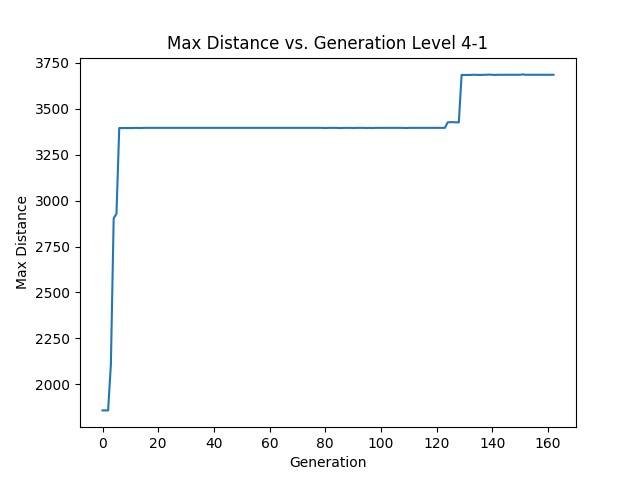
You can see that Mario learns to wait until the piranha plant goes below a certain height and then decides to jump over. One of the really great things about this is since it started training on generation 1216 for level 4-1, it only took 129 generations for it to learn how to to beat the level. I continued having that population train to see if different generations would optimize their solution. In this case they did not. This is how the max distance changed over time for 4-1:
So what happened with level 2-1? Let’s find out!

Mario was never able to beat this level, but it might be apparent why. That spring is a tricky entity because is has a value of \(-1\). Even if Mario generalizes enemies across all inputs he may never jump the way he needs to on the spring. It requires holding “A” to get a large jump. Not only that but Mario would need to learn that jumping on all enemies is good or learn that only jumping on enemies at a certain block is good. It’s possible that given enough time he would be able to overcome this, but I didn’t continue training. A really cool thing is this Mario also learned to wait until the piranha plant goes below a certain height. Remember, these are all different populations, so it’s cool to see different populations come to similar solutions for the same problem.
Now let’s take a look at the first 296 generations. Because these individuals helped shape the other AI, it’s important to see how we got here:
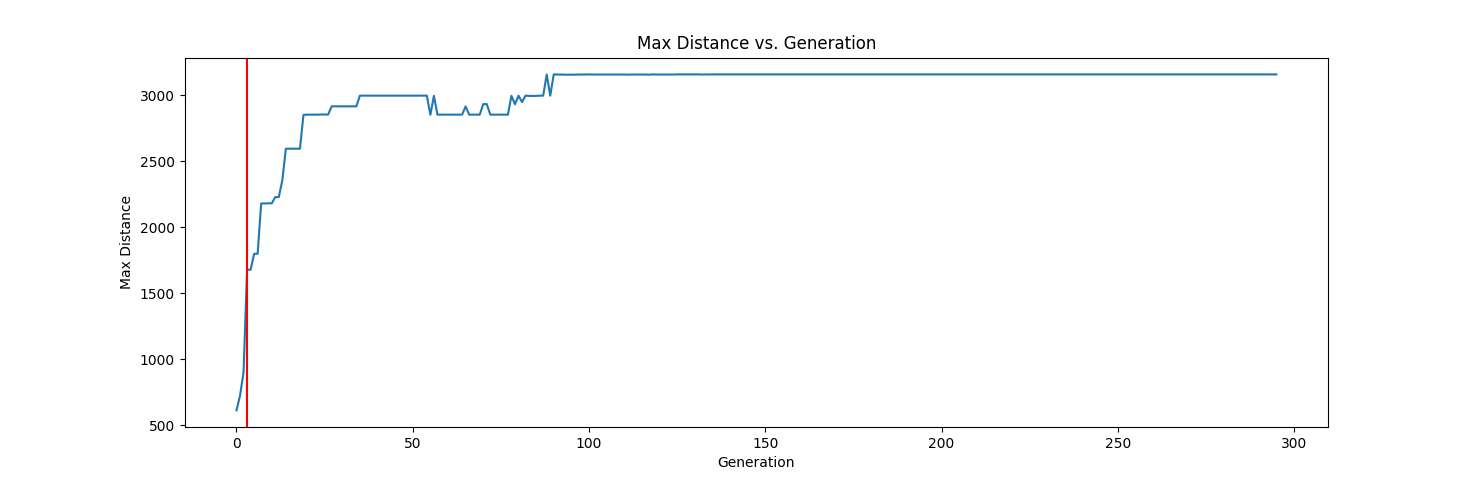
Hopefully you notice the red line. This is where the population changed. Originally I started with a selection mechanism (200+1000) with infinite lifespan. This means that the best 200 individuals get carried over each generation and 1000 offspring are produced, resulting in 1200 total individuals. This causes the max distance to never drop from one generation to the next because the 200 best individuals get carried over. In early generations this can help ensure the fittest survive. Once the population became stagnant for a certain number of generations, the selection mechanism changes to (10,90). Instead of carrying over the best individuals, this mechanism only produces offspring. Because of this there is no guarantee that the maximum distance strictly increases. You can see this throughout after the red line. Here, 10 would be the number of parents. This doesn’t matter since the value would only be set on the first generation. The number of offspring was also reduce from 1000 to just 90 to help generations run faster. Normally you can keep this number the same, but since my computer isn’t the fastest, I chose to kill off a bunch of AI randomly instead.
Limitations of Genetic Algorithms
I just spent a good amount of time showing how genetic algorithms can be used for evolving an AI, and ultimately having it learn in complex environments. There are some issues, however, using this approach. One issue that you may have noticed already is the need to define a fitness function. With a good fitness function the AI can learn an environment quite well, but with a poor fitness function an AI may never actually learn the environment. Let’s change the fitness function to this:
def fitness(frames, distance, did_win, game_score):
    return max(distance ** 1.9 - \
           frames ** 1.5 +   \
           min(max(distance-50, 0), 1) * 2000 + \
           game_score**2.2 + \
           did_win * 1e6, 0.00001)
In this case whatever Mario gets as a score in the actual game is rewarded greatly. Here is how this plays out:

Notice how Mario decides to just hit every block in hopes that the score increases. Because the overall game score is increasing, this means Mario gets around 9.7 million fitness just from the game score! In order to have the distance provide a similar score, Mario would need to go 4759 distance, but the level is only around 3600! Because of this Mario is never going to really learn to optimize for distance.
Another issue with genetic algorithms is they learn at the end of an episode. In fact, I’m calculating fitness at the end of the episode. Fitness could be calculated at each timestep but this also has issues. Imagine calculating fitness at each timestep. If Mario is unable to progress in the level due to an enemy blocking the path, the fitness will drop since the amount of time Mario is alive has increased, while the distance traveled is unchanged. In this case what do you do? Kill off Mario because fitness is decreasing? It’s a complicated problem for genetic algorithms. When you calculate fitness at the end of an episode, you don’t need to worry about that. So what’s the problem with calculating it at the end? Well, the AI is only rewarded at the end and everything in the middle doesn’t really matter. Imagine training a self driving car using a genetic algorithm, where the goal is to get you to work as fast as possible. The fitness function could look like this:
def fitness(time_taken):
    return MAX_TIME - time_taken
Remember, genetic algorithms only know how well they did at the end. In this case it might change what’s done in the middle to maximize the fitness it will get. But what if there’s a red light? The fitness function doesn’t know about red lights and the AI might learn to run them to maximize the fitness. We should take that into account:
def fitness(time_taken, red_lights_ran):
    if red_lights_ran > 0:
        return 0.0  # Bad AI
    return MAX_TIME - time_taken
Now we don’t need to worry about red lights. But what if a kid is crossing the street illegally where there isn’t a light? Does the genetic algorithm say it should stop? No. In fact, the genetic algorithm just wants that sweet, sweet fitness, so it might hit the child. Let’s fix that in the fitness function:
def fitness(time_taken, red_lights_ran, kids_hit):
    if red_lights_ran > 0 or kids_hit > 0:
        return 0.0  # Bad AI
    return MAX_TIME - time_taken
This type of thinking can go on for a while. But even if you create the perfect fitness function we will still have a problem. The genetic algorithm learns at the end of an episode. This means it doesn’t know running the red light or hitting the kid is bad until it does it and gets a low fitness! In fact, the genetic algorithm won’t even realize that driving at a child is bad until it hits them. It doesn’t have a concept of when it’s about to do something bad.
Conclusion
In this post I covered quite a bit. I’ve talked about benefits of genetic algorithms and how they can be used to search high dimensional problems. I discussed how to use a neural network as a function approximator. I described states and what they look like in Super Mario Bros and how to read those values from RAM. You should also now understand how generalization and discrimination between states can help reduce high dimensional problems. After all of that I discussed how to define a fitness function and finally how to combine everything to create an AI that learns to solve levels in Super Mario Bros. You’ve seen the effects of this and know the limitation. These limitations are crucial becasue they are what other algorithms address. The combination of genetic algorithms and neural networks are powerful but also limited. In future posts I will talk about some of the algorithms that build off similar ideas and how they can be used to solve fun and challenging environments. Hopefully you enjoyed the content. If you have any feedback, I’d love to hear it!